
One of the assumptions of a multiple regression is that the independent variables are independent of each other, that there is very little relationship among the variables or no collinearity. What happens when you want to work with a set of independent variables where you know there are relationships among them and sometimes very strong relationships? One approach is to pick and choose which variables to include and try to develop the best regression from there. However, you may be missing out on some very key relationships by doing this. Another option is to run a Ridge Regression.
Ridge regression is a form of regression where you add a degree of bias and thus reduce the standard errors of the regression coefficients. Another biased regression technique is principal components regression.
This post will concentrate on Ridge Regression. Also PLEASE NOTE that for a more statistically minded approach to this procedure please review a statistics textbook or paper. These notes are my interpretation and by no means complete.
The first step in performing a ridge regression is to standardize the variables, both independent and dependent, by subtracting their means and dividing by their standard deviations. This allows all calculations to be based on the standardized variables, however, most statistical packages will present the results in the original scale. So no worries about changing them back.
With ridge regression, what happens is that you are changing the diagonals of the correlation matrix, which would normally be 1, by adding a small bias or a k-value. This is where the name ridge regression came from, since you are creating a “ridge” in the correlation matrix by adding a bit to the diagonal values. Choosing a starting value for k can be tricky and deciding when to stop can be as tricky. Rules of thumb to consider:
- use a Ridge Trace plot to help visualize where the regression coefficients stabilize
- choose the smallest value of k after the regression coefficients stabilize
- choose the smallest value of k possible – since this will introduce the smallest bias
- as k increases, the regression coefficients will eventually drive to 0
As a ridge regression is performed the analysis will calculate a VIF or variance inflation factor. The rule of thumb is to use a cut-off value of 10 for the VIF. What does this mean? If you work through the calculations of a ridge regression, a VIF of 10 or greater translates to an R-squared value of 0.90, which means that at least one independent variable is highly correlated to the remaining independent variables and you are back to dealing with multicollinearity in your dataset.
Phew… now that you have some idea or I hope a better idea as to what Ridge Regression is all about let’s now see how we run one in SAS. We will use a dataset from a research group at the University of Guelph as an example. Please note that only the coding and results will be shown in this post.
Ridge Regression in SAS
With this sample dataset we are looking at the relationships among the following soil parameters:
- Cation Exchange Capacity (CEC)
- pH of the soil (pH)
- Organic matter (OM)
- CEC x pH
- OM x pH
- Relative Extractable Nickel (RelExtNi)
Step 1: Correlation Analysis
Perform a correlation analysis to determine whether there are strong relationships among the variables. Remember that the presence of collinearity or multicollinearity is one of the main reasons we are looking to run a ridge regression.
Proc corr data = soil;
var CEC pH2007 OM ExtNi RelExtNi;
Run;
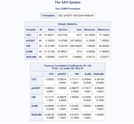
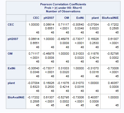
By reviewing these correlations – you can see that there are indeed significant relationships among the independent variables.
Step 2: Ridge Regression Analysis
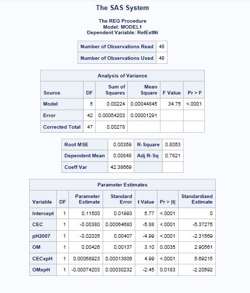
Proc reg data=soil outest=b outvif ridge=0 to 0.048 by .004;
model RelExtNi = CEC pH2007 OM CECxpH OMxpH/STB;
Run;
- Proc reg: calls on the PROCedure to run regression
- outest = b: will create a dataset called b with the model estimates and any additional requested statistics
- outvif: outputs the VIF or variance inflation factors to the outest= dataset
- ridge = 0 to 0.048 by 0.004: performs the ridge regression where your k-value will start at 0, go to 0.048 by increments of 0.004
- model RelExtNi = CEC pH2007 OM CECxpH OMxpH/STB; Our model is RelExtNi = CEC + pH2007 + OM + CECxpH + OMxpH
- STB: displays the standardized parameter estimates
Step 3: Output Review
Regression output
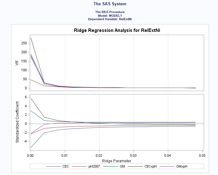
Ridge Trace Plot
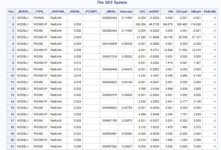
To view the contents of the b dataset which contains the estimates and VIF – use the following:
Proc print data=b;
Run;
Step 4: Selecting your estimates
Recall the Rules of thumb to consider:
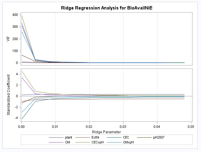
- use a Ridge Trace plot to help visualize where the regression coefficients stabilize
In our output this appears to occur after 0.01 – maybe 0.012
- the VIF rule of thumb is to use a cut-off value of 10
By looking at our output from the b dataset – this appears to be the case with a _ridge_ value of 0.012.
For this example, the most appropriate estimates, with minimum amount of bias (k=0.012 this is the bias) and where we reduce the multicollinearity in our dataset (VIF < 10 means that our R-squared is less than .90 among our independent variables) are:
RelExtNi = 0.04470 – 0.001*CEC -0.00538* pH + 0.001* OM + 0 * CEC x pH + 0 * OM x pH
This essentially removed the interactions and provided more realistic and expected results.
Let’s take a look at a second example. Same dataset, but now we are looking at bioavailability of extractable Ni (BioAvailNiE).
Additional variables include:
- plant nickel (plant)
- extractable nickel (ExtNi)
Step 1: Correlation Analysis
Step 2: Ridge Regression Analysis
Proc reg data=soil outvif outest=b ridge=0 to 0.048 by .004;
model BioAvailNiE = plant ExtNi CEC pH2007 OM CECxpH OMxpH;
Run;
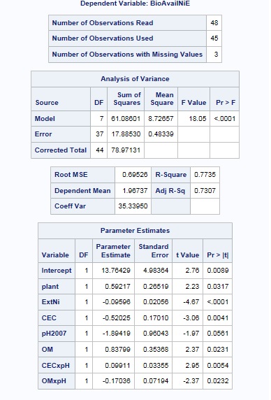
Step 3: Output Review
Regression output
Ridge Trace chart
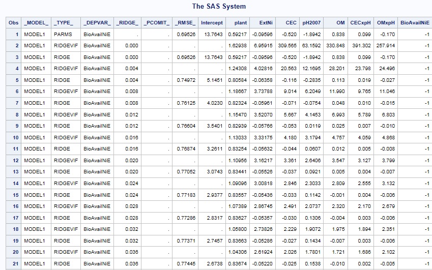
To view the contents of the b dataset which contains the estimates and VIF – use the following:
Proc print data=b;
Run;
Step 4: Selecting your estimates
If you observe the output of the b dataset, you’ll notice that the VIFs are below 10 where _RIDGE_ = 0.012
Selected results provide the following model:
BioAvailNiE = 3.54 + 0.829 * plant -0.058 * ExtNi -0.053 * CEC + 0.0119 * pH + 0.025 * OM + 0.007 * CEC x pH -0.010 * OM x pH
Closing Remarks
If you have used Ridge regression in your analysis, please add a comment to this post. We would love to see different applications and further interpretations of the analysis.

